Understanding Optimal State Estimation
In autonomous systems engineering—whether self-driving cars, spacecraft guidance computers, or warehouse robotic arms—knowing the exact position, velocity, and orientation of your hardware is critical. Unfortunately, real-world sensors are heavily compromised by noise:
- GPS trackers provide correct absolute coordinates but update slowly and jump around (high-frequency noise).
- Inertial measurement units (IMUs) update extremely fast but accumulate mathematical integration drift over time, causing errors to snowball.
The ultimate solution is the Kalman Filter. Originally developed by Rudolf E. Kálmán in 1960 for the Apollo space flight program, the Kalman Filter is a statistically optimal estimator that merges noisy sensor streams mathematically to compute the absolute "ground truth" state.
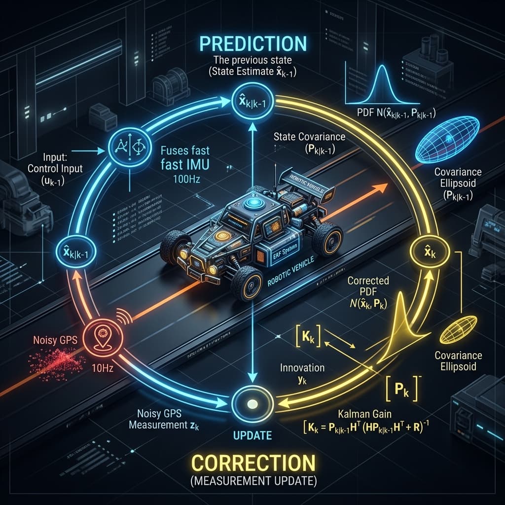
The Dynamic Prediction-Correction Loop
The Kalman Filter executes a recursive, two-step mathematical loop continuously:
Step 1: The Prediction Phase (Time Update)
The filter projects the state forward in time using a mathematical model of physical dynamics (e.g. `distance = speed * time`).x_predicted = F * x_previous + B * uHere, **x** is the state estimate vector, **P** is the error covariance matrix (representing uncertainty), **F** is the state transition matrix, and **Q** is the process noise covariance. With each prediction, uncertainty (**P**) naturally grows.
P_predicted = F * P_previous * F^T + Q
Step 2: The Correction Phase (Measurement Update)
As soon as a new sensor measurement (**z**) arrives, the filter compares it to the predicted state, computes the **Kalman Gain (K)**, and updates the state.K = P_predicted * H^T * (H * P_predicted * H^T + R)^-1Here, **K** represents the trust scaling factor (the Kalman Gain). If sensor noise (**R**) is near zero, **K** approaches 1, meaning we trust the sensor completely. If sensor noise is massive, **K** approaches 0, meaning we ignore the sensor and trust the physics model instead.
x_corrected = x_predicted + K * (z - H * x_predicted)
P_corrected = (I - K * H) * P_predicted
Mistakes to Avoid in Sensor Fusion
❌ Hardcoding process covariance (Q) as static without calibration
The process noise matrix (Q) represents structural model inaccuracies (like wind drift or mechanical slip). Tuning Q too small causes the filter to trust its model blindly, leading to tracking lag. Tuning Q too large makes the filter jump with raw sensor noise. Q must be empirically tuned under real operating loads.
❌ Running dense matrix inversions on low-end 8-bit MCUs
Computing the Kalman Gain requires real-time matrix inversions (solving `H * P * H^T + R` inverse). Attempting multi-dimensional floating-point matrix inversions at 100Hz on an 8-bit Arduino will lock up the CPU completely. Use 32-bit microcontrollers with high-performance float processing (like ESP32 or STM32) or implement pre-calculated static gains.
Frequently Asked Questions
Is a Kalman Filter a low-pass filter?
Not exactly. While it behaves similarly to a low-pass filter by smoothing noisy data, it is a dynamic estimator. It models physical dynamics (acceleration, inertia) to "predict" where the device should be, making it significantly more advanced and responsive than passive low-pass filters.
How do I determine the measurement noise covariance (R)?
R is usually determined experimentally. Place your sensor static on a table, collect 1000 readings, and compute the mathematical variance. This computed variance serves as your baseline input for the R matrix.
What is the Unscented Kalman Filter (UKF)?
The Unscented Kalman Filter is a highly advanced estimator for non-linear systems. Instead of linearizing using complex Jacobian calculus (like the EKF), the UKF selects a minimal set of sample points (sigma points) around the mean, maps them through the actual non-linear equations, and computes the new mean and covariance.
Conclusion
The Kalman Filter is the mathematical cornerstone of modern robotics. By balancing time-based predictions against real-world sensor updates, it delivers clean, optimal state tracking for self-driving vehicles and robotic controllers alike. Implement these algorithms in our Autonomous Vehicles roadmap to see them in action!