How PID Controllers Work: Proportional, Integral & Derivative Control Explained

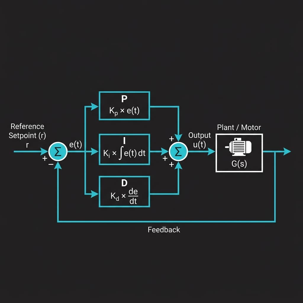
The Closed-Loop Control Concept

Imagine trying to drive a car at exactly 60 km/h. A human driver watches the speedometer (measures output), compares it to the target (setpoint), and adjusts the throttle (corrective output). This is a closed-loop feedback system — and a PID controller does this mathematically, hundreds or thousands of times per second.

The three terms each provide a different dimension of correction:

• P — Proportional: React now. Correct proportional to how wrong you are at this moment.
• I — Integral: Remember the past. Correct for persistent error that P alone cannot eliminate.
• D — Derivative: Predict the future. Slow down your correction if you are approaching the target rapidly, preventing overshoot.

Proportional Term (P): React to Current Error

The proportional output is simply the error multiplied by gain Kp:

P_out = Kp × error

Increasing Kp makes the controller more aggressive — faster response but tends toward oscillation. A Kp that is too high will cause the system to oscillate around the setpoint indefinitely. A Kp that is too low produces a sluggish response with significant steady-state error (called "droop" or "offset").

Integral Term (I): Eliminate Steady-State Error

The integral term sums all past errors over time. Even a tiny sustained error will accumulate, growing the I term until the output is large enough to eliminate the offset:

I_out = Ki × Σ(error × dt)    // Discrete sum in microcontrollers

Integral Windup: A major hazard in real systems. If the actuator saturates (motor at 100% but setpoint not reached), the integrator keeps growing enormous. When the setpoint is finally reachable, the massive accumulated I term causes wild overshoot. Solutions include clamping the integral value or pausing integration during saturation.

Derivative Term (D): Predict Future Error

The derivative term measures how quickly the error is changing and applies a braking force proportional to that rate:

D_out = Kd × (error - previous_error) / dt

Think of Kd as the "brakes" of the PID. If you are approaching the setpoint very fast (error dropping rapidly), D applies a large opposing force, slowing correction before you overshoot. D is also very sensitive to measurement noise — sensor noise creates large dI/dt spikes, so a low-pass filter on the measurement is recommended when using high Kd.

PID Step Response: Visualising Each Term

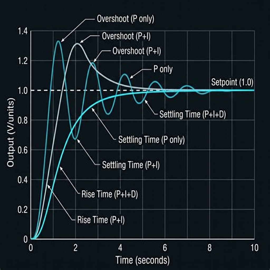
Fig 1: Step response comparison — P only oscillates, P+I overshoots, P+I+D settles smoothly

Arduino PID Implementation

// Simple PID motor speed controller
// Encoder measures actual RPM, output drives PWM to motor driver

float Kp = 2.0, Ki = 0.5, Kd = 0.1;
float setpoint = 150.0; // Target RPM
float integral = 0, prevError = 0;
unsigned long lastTime = 0;

float pidCompute(float measured) {
  unsigned long now = millis();
  float dt = (now - lastTime) / 1000.0; // seconds
  if (dt <= 0) return 0;
  lastTime = now;

  float error = setpoint - measured;
  integral += error * dt;
  integral = constrain(integral, -100, 100); // Anti-windup clamp

  float derivative = (error - prevError) / dt;
  prevError = error;

  float output = Kp*error + Ki*integral + Kd*derivative;
  return constrain(output, 0, 255); // PWM range
}

void loop() {
  float rpm = readEncoderRPM(); // Your encoder reading function
  int pwm = (int)pidCompute(rpm);
  analogWrite(motorPin, pwm);
  delay(10); // 100 Hz control loop
}

Ziegler-Nichols PID Tuning Method

The Ziegler-Nichols method is the most widely taught systematic tuning approach:

1. Set Ki = 0 and Kd = 0. Increase Kp from zero until the system output oscillates with constant, sustained amplitude. Record this as the Ultimate Gain (Ku).
2. Record the oscillation period as the Ultimate Period (Pu) in seconds.
3. Apply Ziegler-Nichols formula: Kp = 0.6Ku, Ki = 1.2Ku/Pu, Kd = 0.075Ku×Pu
4. Fine-tune: if overshoot is too large, reduce Ki. If response is too slow, increase Kp. If oscillating, increase Kd.

Frequently Asked Questions